How AutoTune works
Introduction
AutoTune, the famous pitch correction software released in 1997, is very interesting from a technical point of view. I’ve always thought AutoTune has a very musical quality and can sound very beautiful when applied well. It can add a pleasant rattling quality to a singing voice and can be very expressive and emotional, adding inhuman vibrato, voice cracks, harmonies, etc. Lately, I’ve become interested in how it works, and it turns out it’s actually quite clever. I thought the best way to really understand it is to roll my own and communicate what I learned.
The original patent filed in October 1998 explains everything, but it’s a little verbose, and the language is somewhat cryptic at times. I thought it would be nice to put together an explanation that’s hopefully a little more succinct and clearer. This also gives me the chance to highlight some practical considerations I ran into during the implementation, like error accumulation, that don’t show up in the patent. To support the explanation, I created my own interactive, visual version of the input side of AutoTune embedded in this post that shows the internals of the algorithm as it’s running.1
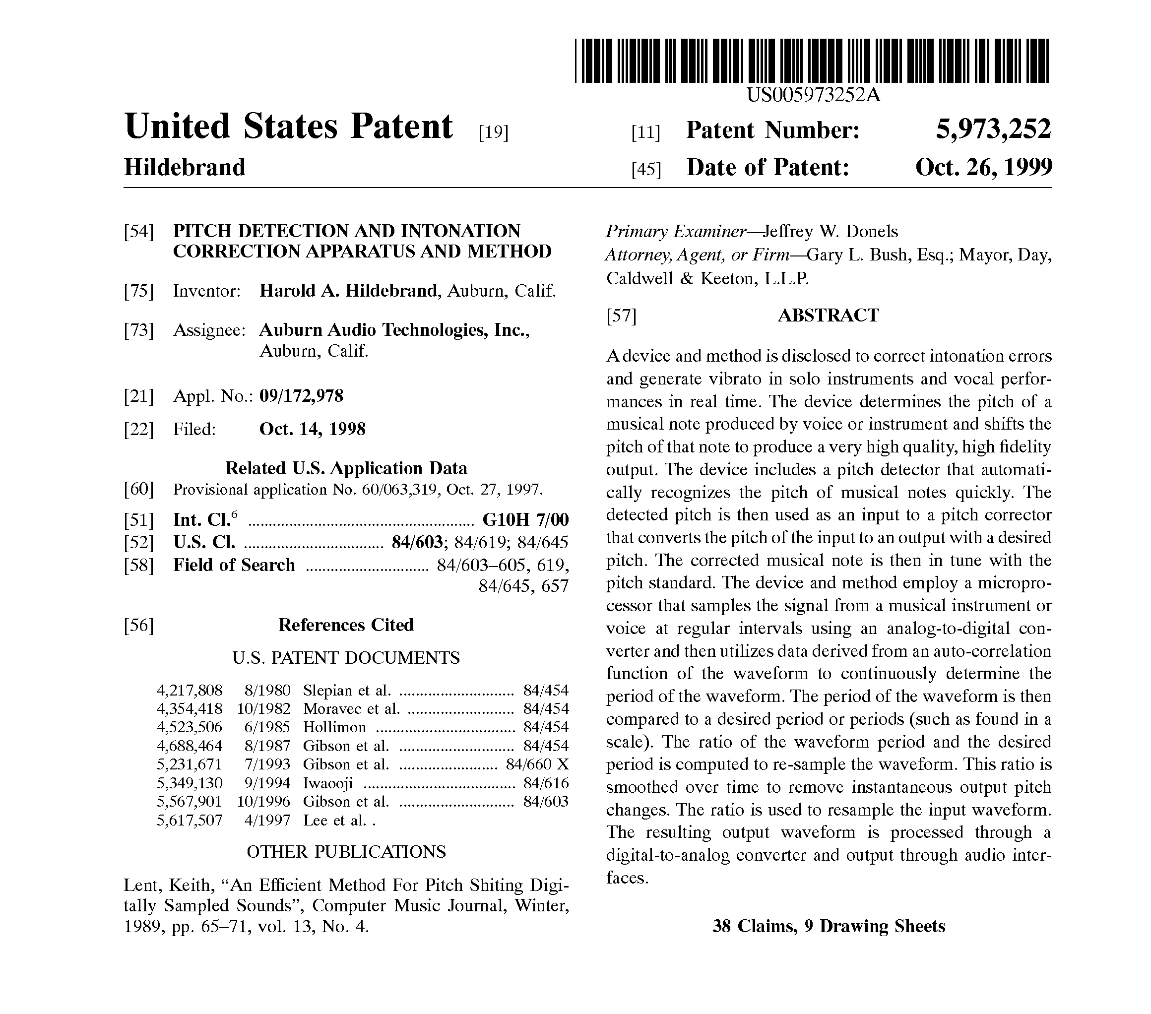
Title page of the AutoTune patent.
Input and output sections
AutoTune can be neatly partitioned into an input and an output section: the input section detects and tracks the pitch of an incoming monophonic musical signal (like a singing voice), and the output section uses that pitch information to output a pitch-corrected version of the input signal. AutoTune can be configured so that the target pitch depends on the tracked pitch (for example the closest neighboring note in a musical scale), or it can be specified explicitly, for example by a MIDI instrument. The output section replays the input audio faster or slower to bring the output pitch closer to the target pitch.2 This post touches only on the input section, which contains most of the richness and technically interesting aspects, with the output section being comparatively simple. In the future, I’ll probably extend the AutoTune demo to include the output section and treat it in a separate post.
Autocorrelations and energies
AutoTune takes its name from autocorrelation: a measure of the correlation of a signal with a time-delayed version of itself, useful for discovering periodicities. The usual definition of the autocorrelation $H^L$ of a real-valued, deterministic signal $x_n$ with domain $\mathbb{Z}$ for a lag value $L \in \{1, 2, \ldots\}$ is
$$ H^L \overset{\text{def}}{=} \sum_{k\in\mathbb{Z}} x_{k} x_{k - L}. $$$H^L$ is then a measure of how correlated the signal $x_n$ is with a version of itself delayed by $L$ samples. This definition assumes the signal has finite energy, which implies that the above sum converges. Note that $H^L$ has no time dependence: it depends only on the signal $x_n$ and the lag value $L$.
In order to detect local, short-lasting periodicities in a signal as it streams in, with the ultimate aim of tracking the pitch of a musical signal over time, it’s natural to introduce a time dependence. To this end, AutoTune uses a modified definition of the autocorrelation that depends on the time index $n$ and sums over only a finite window of samples preceding and including $n$:
$$ H_n^L \overset{\text{def}}{=} \sum_{k=0}^{L - 1} x_{n - k} x_{n - k - L}. $$In words, we can describe $H_n^L$ as the dot product of the $L$ samples immediately preceding (and including) the time index $n$ with the $L$ samples preceding those samples. Note that the window size is tied to the lag value $L$, ensuring maximum time resolution. AutoTune also defines an energy quantity $E_n^L$ in a similar way:
$$ E_n^L \overset{\text{def}}{=} \sum_{k=0}^{2 L - 1} x_{n - k}^2. $$$E_n^L$ is just the energy of the $2 L$ samples preceding (and including) the time index $n$. From here, the following condition can be used as a heuristic for whether the signal $x_n$ is $L$-periodic at time index $n$:
$$ E_n^L - 2 H_n^L \leq \epsilon E_n^L $$where $0 < \epsilon < 1$ is a small, dimensionless threshold value set by the user. One can very loosely understand the left-hand side quantity $E_n^L - 2 H_n^L$ as the amount of energy left over in the previous $2 L$ samples preceding the time index $n$ after subtracting the energy due to $L$-periodicity. If this remaining energy is very small in comparison to the total energy in those samples, we can suppose that there is a significant amount of $L$-periodicity at time $n$. Note that the left-hand side quantity is always $\geq 0$, which will become clear with the following explanation.
The periodicity heuristic also has an intuitive geometric interpretation. To see how, let
$$ \mathbf{x}_n^p \overset{\text{def}}{=} \begin{bmatrix} x_{n-L+1}, \, x_{n-L+2}, \, \ldots, \, x_{n} \end{bmatrix}^\top $$be the $L$ samples immediately preceding (and including) the time index $n$ ($p$ stands for “previous”), and let
$$ \mathbf{x}_n^{pp} \overset{\text{def}}{=} \begin{bmatrix} x_{n-2L+1}, \, x_{n-2L+2}, \, \ldots, \, x_{n-L} \end{bmatrix}^\top $$be the $L$ audio samples immediately preceding those samples. Then
$$ H_n^L = \mathbf{x}_n^p \cdot \mathbf{x}_n^{pp}, $$and
$$ E_n^L = \mathbf{x}_n^p \cdot \mathbf{x}_n^{p} + \mathbf{x}_n^{pp} \cdot \mathbf{x}_n^{pp}. $$Note that, by the distributive property of the dot product,
$$ \begin{aligned} E_n^L - 2 H_n^L &= \overbrace{\mathbf{x}_n^p \cdot \mathbf{x}_n^{p} + \mathbf{x}_n^{pp} \cdot \mathbf{x}_n^{pp}}^{E_n^L} - 2 \, \overbrace{\mathbf{x}_n^p \cdot \mathbf{x}_n^{pp}}^{H_n^L} \\ &= (\mathbf{x}_n^p - \mathbf{x}_n^{pp}) \cdot (\mathbf{x}_n^p - \mathbf{x}_n^{pp}), \end{aligned} $$which is of course $\geq 0$. The periodicity condition can then be written as
$$ \underbrace{(\mathbf{x}_n^p - \mathbf{x}_n^{pp}) \cdot (\mathbf{x}_n^p - \mathbf{x}_n^{pp})}_{E_n^L - 2 H_n^L} \leq \epsilon \underbrace{(\mathbf{x}_n^p \cdot \mathbf{x}_n^{p} + \mathbf{x}_n^{pp} \cdot \mathbf{x}_n^{pp})}_{E_n^L}, $$or, equivalently,
$$ \frac{(\mathbf{x}_n^p - \mathbf{x}_n^{pp}) \cdot (\mathbf{x}_n^p - \mathbf{x}_n^{pp})}{\mathbf{x}_n^p \cdot \mathbf{x}_n^p + \mathbf{x}_n^{pp} \cdot \mathbf{x}_n^{pp}} \leq \epsilon. $$The left-hand side of the above inequality can be seen as a kind of dimensionless distance measure between the previous $L$ samples and the $L$ samples preceding those samples. When they are very similar (as in the case of high $L$-periodicity), the distance is close to zero, and when they are very different (as in the case of low $L$-periodicity), the distance is close to 2.3
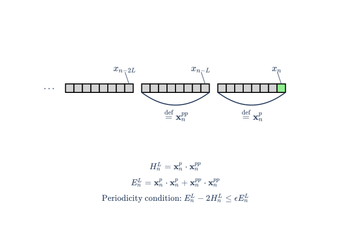
The core of the AutoTune pitch detection and tracking: to roughly determine whether the signal $x_n$ is locally $L$-periodic at time index $n$, we compare the local autocorrelation $H_n^L$ to the local energy $E_n^L$. The most recently acquired sample, $x_n$, is highlighted in green. The calculation is repeated for many candidate lag values $L$ as each new sample arrives.
Fast update equations
The trick is that $H_n^L$ and $E_n^L$ can be updated quickly in a streaming setting using the following recurrence relations:
$$ H_n^L = H_{n - 1}^L + x_n x_{n - L} - x_{n - L} x_{n - 2 L} $$and
$$ E_n^L = E_{n - 1}^L + x_n^2 - x_{n - 2 L}^2. $$In words, to calculate $H_n^L$ and $E_n^L$ for the next sample, we can just add a term for the new sample (time index $n$) and subtract a term for the old sample (time index $n - 2 L$) that just went out of bounds. So as new samples come in, there’s no need to recalculate the entire sums. This convenient property contrasts this approach from Fourier-based or Wavelet-based methods, which can’t be quickly updated in this way.4 This is the main trick behind AutoTune, about which its inventor, Andy Hildebrand, said:
I realized that most of the arithmetic was redundant, and could be simplified… My simplification changed a million multiply adds into just four. It was a trick—a mathematical trick.
We’ve explored the general principle of how AutoTune works, but understanding how this principle is actually used to detect and track the pitch of a musical signal $x_n$ requires a few more considerations.
Pitch detection and tracking
AutoTune is set up as a state machine with exactly two states: detection mode and tracking mode. In detection mode (which is the mode AutoTune is in at startup), AutoTune hasn’t detected any pitch yet and is constantly listening for it. Once a pitch is detected, AutoTune enters tracking mode. Here, AutoTune tracks the detected pitch until the track is lost, at which time it switches back to detection mode.
The reason for the split is a matter of tradeoff and computational feasibility. Detection mode needs to cover a wide range of frequencies (like the entire human vocal range). In order to make this work,5 it consumes a downsampled version of the input audio, reducing the computational cost, but also the time and frequency resolution. While this is good enough for detection, once a pitch is detected, the tracking needs to work with a much finer resolution in order to accurately track fast and subtle modulations in the pitch across its lifetime. To make this work, tracking mode consumes the full resolution audio stream, but covers only a rather small window of frequencies surrounding the currently tracked pitch.
To make this more explicit, let’s explore each of these modes in detail.
Detection mode
Detection mode has the job of listening to the input audio and detecting its fundamental pitch without accidentally identifying a harmonic or an integer multiple of the true lag (see below for a more detailed discussion of these pitfalls). It works by updating arrays of $H_n^L$ and $E_n^L$-values using the fast update equations for a large range of $L$-values as each new input sample arrives. The $L$-values, which refer to lag times measured in audio samples, cover every integer in a range determined by a user-configured minimum and maximum detection frequency. The recommended values for this from the patent are 50.1 Hz and 2756 Hz respectively, covering the human vocal range. As noted above, detection mode works on a (usually around 8x) downsampled version of the input audio stream for performance reasons.
After the $H_n^L$ and $E_n^L$-arrays are updated to reflect the new sample, the $L$-values are then searched in ascending order for the first one, call it $L_{\text{min}}^{(1)}$, that satisfies the periodicity condition $E_n^L - 2 H_n^L \leq \epsilon E_n^L$. Searching in ascending order is intentional because, for example, if $L$ is a period of the audio, then so is every integer multiple of $L$, and we want to avoid these spurious detections.
If no such $L$-value is found, we simply stay in detection mode and move onto the next input sample. Otherwise, it’s possible that the $L$-value found actually corresponds to the first harmonic (which is approximately double the fundamental frequency) instead of the fundamental. To determine this, we check whether the lag value $2 L_{\text{min}}^{(1)}$ is outside of the detectable range determined by the user-configured minimum detection frequency. If it is, we simply report $L_{\text{min}}^{(1)}$ as the detected lag and enter tracking mode. Otherwise, we find the next $L$-value greater than $L_{\text{min}}^{(1)}$, call it $L_{\text{min}}^{(2)}$, that satisfies the periodicity condition. If none is found, we stay in detection mode and move onto the next input sample. Otherwise, we compare the $(E_n^L - 2 H_n^L)$-score of $L_{\text{min}}^{(1)}$ versus $L_{\text{min}}^{(2)}$ on the full-resolution audio, entering tracking mode with whichever of these two $L$-values has the better (lower) score.
Tracking mode
Once in tracking mode, AutoTune attempts to track the current pitch as far as it can until the track is lost, at which time it switches back to detection mode. Tracking mode consumes the full-resolution audio and works similarly to detection mode: when a new sample arrives, arrays of $H_n^L$ and $E_n^L$-values are updated using the fast update equations to incorporate the new sample.6 These arrays are much shorter, covering only a narrow window of $L$-values surrounding the currently tracked pitch. The $L$-values cover every integer in the range determined by the tracking window’s position and size. The window position moves up and down depending on the tracked pitch according to the rule described below, while the window size is a fixed parameter set by the user.
Once every few samples (with the exact number being set by the user but recommended by the patent to be 5), after the arrays are updated, the $L$-value with the smallest $(E_n^L - 2 H_n^L)$-score is calculated. If this $L$-value is at the edge of the tracking window or doesn’t satisfy the periodicity condition $E_n^L - 2 H_n^L \leq \epsilon E_n^L$, the track is lost, and detection mode is entered. Otherwise, this best $L$-value is further refined via a quadratic interpolation with the $(E_n^L - 2 H_n^L)$-scores of its two neighboring $L$-values.
If the tracked pitch changed from the last update, the tracking window is moved up or down by one index to bring the tracked pitch closer to the middle of the window. The arrays of $H_n^L$ and $E_n^L$-values are appropriately shifted up or down, necessitating the new edge values to be recalculated naively from the definition.
The demo below shows detection mode and tracking mode, together with the tracking window, in action.
Demo
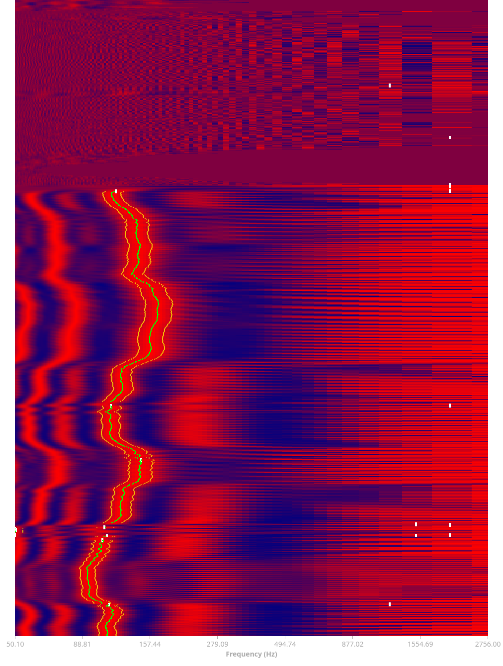
Screenshot of the AutoTune visualization. Note the accuracy of the tracking (green) while following a vocal vibrato. Note also the many spurious detection events (white) that don’t lead to a solid track.
The difficulty of harmonics
Detection mode has the task of detecting the lag $L$ corresponding to the fundamental frequency (if one exists) of the incoming audio without accidentally detecting a harmonic or an integer multiple of $L$. See the appendix for more details on fundamental frequencies and harmonics. To explore this in a simpler setting, consider the case of a pure sine tone:
$$ x_n = \sin(\omega n). $$The autocorrelation $H_n^L$ in response to this signal is known in closed form (derivation in the appendix):
$$ H_n^L = \frac{1}{2} L \cos(\omega L) - \frac{1}{2} \frac{\sin(\omega L) \cos(\omega (2 n - 2 L + 1))}{\sin(\omega)}. $$Similarly, the energy $E_n^L$ is also known in closed form:
$$ E_n^L = L - \frac{1}{2} \frac{\sin(2 \omega L) \cos(\omega (2 n - 2 L + 1))}{\sin(\omega)}. $$Note that these quantities are periodic in $n$, but not in $L$.
From here, we can plot the normalized periodicity score, $(E_n^L - 2 H_n^L) / E_n^L$, versus the lag $L$. For this, we set $\omega$ to correspond to the frequency 220 Hz (A3), which is well within the human vocal range. A realistic sampling rate of 48 kHz is used.
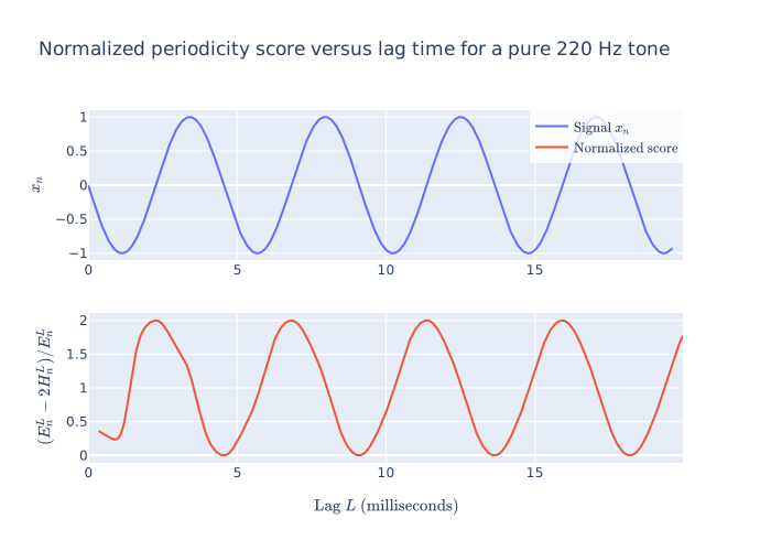
Normalized periodicity score (bottom) for a pure 220 Hz (A3) tone (top). For the sake of this example, we consider the autocorrelation $H_n^L$ and energy $E_n^L$ at time $n = 0$. The normalized periodicity score dips down to zero at integer multiples of the period of the signal (around 4.55 milliseconds) as expected.
This gives an expected result: the normalized periodicity score does its job and approaches zero as $L$ approaches integer multiples of the period, $2 \pi / \omega$, of the signal, which in this case is around 4.55 milliseconds or 218 samples at our 48 kHz sampling rate.
The fact that the score dips at every integer multiple of the period suggests that when scanning the $H_n^L$ and $E_n^L$-arrays for periodicities, it’s better to start with smaller $L$-values and scan upwards in order to avoid accidentally detecting an integer multiple of the period. While this is valid, the situation is complicated by the presence of harmonics. The human singing voice of course isn’t just a single pure tone and has many higher harmonic frequencies mixed in. These usually appear at roughly integer multiples of the fundamental frequency and in various (and changing) proportions. Although the normalized periodicity score is somewhat robust against harmonics and doesn’t usually detect them as strongly as the fundamental, starting the scan for the period from smaller $L$-values (and therefore higher frequencies) carries the risk of accidentally identifying one of these harmonics as the period of the signal. To see how, consider another toy example: this time an equal mix of a 220 Hz (A3) tone, plus two additional tones: 440 Hz and 660 Hz. This is a rough approximation of a fundamental frequency with the first two harmonics added.
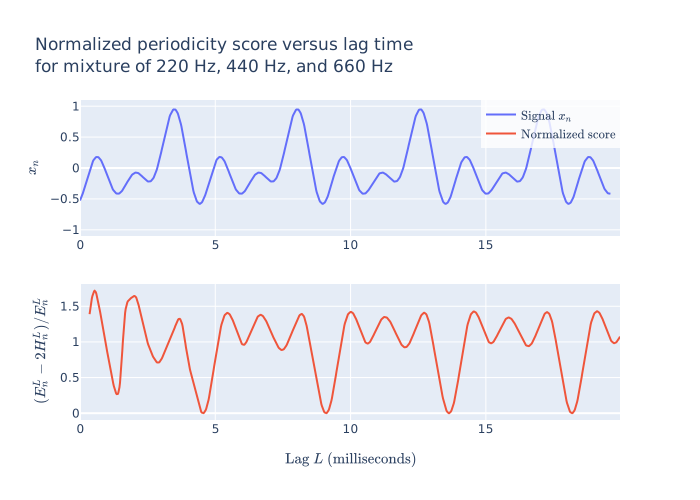
Normalized periodicity score (bottom) for an equal mixture of a pure 220 Hz (A3) tone plus two harmonics: 440 Hz and 660 Hz (top). The relative phase differences for the tones are randomly generated. Again, we arbitrarily consider $H_n^L$ and $E_n^L$ at time $n = 0$. The normalized periodicity score dips down to zero at integer multiples of the period of the 220 Hz fundamental frequency (around 4.55 milliseconds) as expected. The presence of the 440 Hz (period around 2.27 milliseconds) and 660 Hz (period around 1.52 milliseconds) harmonics, however, complicate the detection of the period by causing spurious dips in the score that could be mistaken for the fundamental. These dips are significantly smaller than those associated with the fundamental, and so can be differentiated in this case with a carefully configured detection threshold $\epsilon$.
The fundamental frequency is still of course 220 Hz (period around 4.55 milliseconds) as before, but the 440 Hz and 660 Hz (periods around 2.27 milliseconds and 1.52 milliseconds respectively) harmonics also affect the score with additional dips, albeit less prominently than the true period. This suggests that we should take care when choosing a detection threshold value $\epsilon$ past which we consider the signal to be periodic: if we chose a threshold that’s too lenient, we may accidentally detect a harmonic instead of the fundamental. On the other hand, if we choose a threshold that’s too strict, we may not detect any periodicity at all, particularly in the real-world case of a mostly periodic signal with some noise mixed in. This demonstration also justifies the need for the rather elaborate AutoTune detection algorithm detailed above that compares the periodicity score of a candidate lag $L$ to the score of $2 L$, since it’s possible the former may correspond to the first harmonic, with the latter corresponding to the fundamental.
Error accumulation
When invoking the cumulative $H_n^L$ and $E_n^L$ fast update equations from above thousands of times per second while running AutoTune for minutes or hours at a time, the question of error accumulation arises. As a reminder, the equations are:
$$ H_n^L = H_{n - 1}^L + x_n x_{n - L} - x_{n - L} x_{n - 2 L} $$and
$$ E_n^L = E_{n - 1}^L + x_n^2 - x_{n - 2 L}^2. $$In practice, each time one of these equations is used, a small numerical floating point error is accumulated. To combat this, we can use Kahan summation, which is a method for reducing numerical error when calculating a sum of many floating point numbers.
Consider the simple case of a C function sum_numbers that sums n floating point numbers:
float sum_numbers(const float *numbers, size_t n) {
    float sum = 0.0f;
    for (size_t i = 0; i < n; i++) {
        sum += numbers[i];
    }
    return sum;
}
One might be tempted to reason that, assuming a random input, as we add terms to sum, the roundoff errors essentially form a random walk, with the root mean square of the total accumulated error therefore growing as $\sqrt{n}$. But in reality, as we add terms to sum, the additional roundoff error added by each new term will likely get larger as more terms are added. This is due to a phenomenon in floating point arithmetic known as swamping: the roundoff error of the addition of two floating point numbers is worse the more their magnitudes are different. With Kahan summation, which works by calculating an error for each additional term of the sum and subtracting it from the next term, the additional roundoff error from each new term is guaranteed to be no more than proportional to the absolute value of the new term as long as $n$ doesn’t exceed the reciprocal of the machine epsilon of the error variable.7 Below is the same function written using Kahan summation:
float sum_numbers_kahan1(const float *numbers, size_t n) {
    float sum = 0.0f;
    float error = 0.0f;
    for (size_t i = 0; i < n; i++) {
        float term = numbers[i] - error;
        float new_sum = sum + term;
        float difference = new_sum - sum;
        error = difference - term;
        sum = new_sum;
    }
    return sum;
}
Each time we add a term, we calculate the difference between the new sum and the term we just added. This should be equal to (up to floating point roundoff error) the new term. Any difference between these two is saved in an error variable which is subtracted when adding the next term, and the process repeats itself. The algorithm can be neatly generalized as follows:
void increment_kahan(float *sum, float increment, float *error) {
    float term = increment - *error;
    float new_sum = *sum + term;
    float difference = new_sum - *sum;
    *error = difference - term;
    *sum = new_sum;
}
This can then be used by any code that calculates a sum of many terms. For example, here is the above sum_numbers_kahan1 written in terms of increment_kahan:
float sum_numbers_kahan2(const float *numbers, size_t n) {
    float sum = 0.0f;
    float error = 0.0f;
    for (size_t i = 0; i < n; i++) {
        increment_kahan(&sum, numbers[i], &error);
    }
    return sum;
}
It can also be used to implement an update_autocorrelations function that performs the fast $H_n^L$-update:
void update_autocorrelations(float *autocorrelations,
                             float *prev_autocorrelations,
                             float *errors,
                             const float *new_samples,
                             const unsigned *lags,
                             unsigned n_lags,
                             unsigned n_new_samples) {
    // autocorrelations:       (n_lags, n_new_samples)
    // prev_autocorrelations:  (n_lags,)
    // errors:                 (n_lags,)
    // new_samples:            (n_new_samples,)
    // lags:                   (n_lags,)

    for (unsigned lag_id = 0; lag_id < n_lags; lag_id++) {
        unsigned lag = lags[lag_id];

        for (unsigned sample_id = 0;
             sample_id < n_new_samples;
             sample_id++) {
            float autocorrelation;

            if (sample_id == 0) {
                autocorrelation = prev_autocorrelations[lag_id];
            } else {
                autocorrelation = autocorrelations[sample_id - 1];
            }

            // Include the present term
            float increment1 =
                (new_samples[sample_id]
                 * new_samples[(int) sample_id - (int) lag]);
            increment_kahan(&autocorrelation, increment1, &errors[lag_id]);

            // Subtract the recently out-of-bounds term
            float increment2 =
                -(new_samples[(int) sample_id - (int) lag]
                  * new_samples[(int) sample_id - 2 * (int) lag]);
            increment_kahan(&autocorrelation, increment2, &errors[lag_id]);

            autocorrelations[sample_id] = autocorrelation;
        }

        // Save `prev_autocorrelations` for the next call
        prev_autocorrelations[lag_id] = autocorrelations[n_new_samples - 1];

        // Point to the autocorrelations array for the next lag
        autocorrelations += n_new_samples;
    }
}
The update_energies function for $E_n^L$ is implemented in an analogous way.
We can perform a soak test to roughly simulate how the error accumulation for the $H_n^L$ and $E_n^L$-values behaves after hours of runtime in detection mode when using naive versus Kahan summation. For this, we run the update functions on randomly generated samples from $\text{Uniform}(-1,1)$ with a sampling rate of 6 kHz (consistent with detection mode with 8x downsampling at 48 kHz full resolution) for 48 hours’ worth of audio. The $L$-values used correspond to the range from 50.1 Hz to 2756 Hz, which are the suggested minimum and maximum detectable frequencies from the patent.
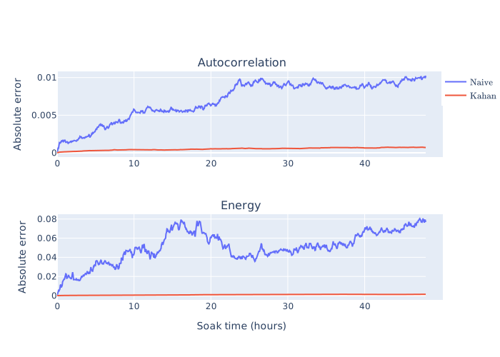
Error accumulation of cumulatively calculated autocorrelations $H_n^L$ (top) and energies $E_n^L$ (bottom) for a realistic range of $L$-values using naive versus Kahan summation running on two days’ worth of random audio. The simulation was run at a realistic 6 kHz sampling rate (consistent with detection mode with 8x downsampling at 48 kHz full resolution). For each time index $n$, the absolute error of the worst $L$-value is shown as compared with the corresponding quantity calculated directly from the definition.
As expected, the naive summation accumulates absolute error much faster than the Kahan summation. To get an idea for the relative error, we can inspect the distributions of relative errors during the final 20 minutes of the 48-hour soak test:
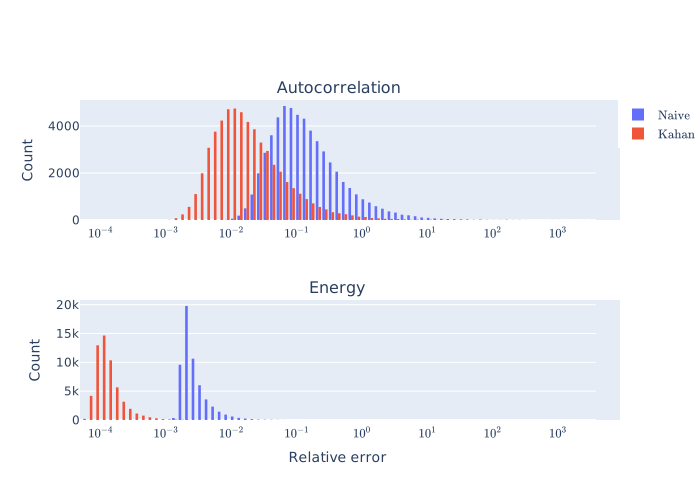
Distributions of relative errors of autocorrelations and energies during the final 20 minutes of the soak test.
The Kahan summation appears to, on average, have a relative error between around 10 and 100 times smaller than naive summation during the final 20 minutes.
Ideas for the future
There’s still plenty more to explore, so this is definitely just the beginning of my AutoTune journey. Some unorganized ideas for the future:
- Extend the demo to include the output side (pitch correction)
- Use the pitch tracking as a game controller for a Pong or Flappy Bird-style game
- Use the pitch tracking to visualize a stabilized waveform of the streaming input audio
Appendix
Brief discussion of harmonics
Any sufficiently well-behaved, $L$-periodic, real-valued signal $x(t)$ is just a weighted sum of the basis functions $\cos(2 \pi n t / L)$ and $\sin(2 \pi n t / L)$ for $n \in \{0, 1, 2, \ldots \}$. Note that these basis functions themselves are also $L$-periodic. Of course, a singing voice isn’t perfectly periodic, but at any given instant, it’s close enough that the following conclusions apply, albeit approximately. A Fourier transform recovers the weights for the basis functions associated with each frequency $f_n = n / L$. The smallest frequency (not including $f_0$, which is just zero) is $f_1 = 1 / L$, which corresponds to the period $L$. This is called the fundamental frequency, which is of course what AutoTune aims to detect and track. The higher frequencies $f_2$, $f_3$, etc, which are usually mixed in with less intensity in the case of naturally produced sounds, are called harmonics. In the case of singing, different vowels (and therefore different vocal tract geometries, which give rise to different combinations of standing wave solutions to the wave equation) correspond to different relative mixtures of these harmonics.
Derivations of $H_n^L$ and $E_n^L$ for a pure tone
Here I’ve put the derivations for $H_n^L$ and $E_n^L$ in response to a sine wave:
$$x_n = \sin(\omega n).$$This is just for completeness and not because it’s that interesting. The strategy for both is basically:
- Write down the definition
- Write the sines in terms of complex exponentials
- After some manipulation, the quantity can be written as a constant plus a sum of cosines
- Write the sum of cosines as a partial sum of a geometric sequence
- Substitute in the well-known formula for the partial sum of a geometric sequence
Derivation of $H_n^L$
From the definition, we have
$$ \begin{gathered} H_n^L = \sum_{k=0}^{L - 1} x_{n - k} x_{n - k - L} \\ = \sum_{n=0}^{L - 1} \sin(\omega (n - k)) \sin(\omega (n - k - L)). \end{gathered} $$For convenience, let
$$ A_{nk} = \omega (n - k) $$and
$$ B_{nk} = \omega (n - k - L). $$Then
$$ \begin{gathered} H_n^L = \sum_{k=0}^{L - 1} \sin(A_{nk}) \sin(B_{nk}) \\ = \sum_{k=0}^{L - 1} \left(\frac{e^{i A_{nk}} - e^{-i A_{nk}}}{2 i}\right) \left(\frac{e^{i B_{nk}} - e^{-i B_{nk}}}{2 i}\right) \\ = -\frac{1}{4} \sum_{k=0}^{L - 1} \left(e^{i (A_{nk} + B_{nk})} - e^{i (A_{nk} - B_{nk})} - e^{-i (A_{nk} - B_{nk})} + e^{-i (A_{nk} + B_{nk})}\right) \\ = -\frac{1}{4} \sum_{k=0}^{L - 1} \left(e^{i (A_{nk} + B_{nk})} + e^{-i (A_{nk} + B_{nk})} - \left(e^{i (A_{nk} - B_{nk})} + e^{-i (A_{nk} - B_{nk})}\right)\right) \\ = -\frac{1}{2} \sum_{k=0}^{L - 1} \left(\frac{e^{i (A_{nk} + B_{nk})} + e^{-i (A_{nk} + B_{nk})}}{2} - \frac{e^{i (A_{nk} - B_{nk})} + e^{-i (A_{nk} - B_{nk})}}{2}\right) \\ = -\frac{1}{2} \sum_{k=0}^{L - 1} \left(\cos(A_{nk} + B_{nk}) - \cos(A_{nk} - B_{nk})\right) \\ = \frac{1}{2} \sum_{k=0}^{L - 1} \cos(A_{nk} - B_{nk}) -\frac{1}{2} \sum_{k=0}^{L - 1} \cos(A_{nk} + B_{nk}). \end{gathered} $$Substituting back in the formulas for $A_{nk}$ and $B_{nk}$ then gives
$$ \begin{gathered} H_n^L = \frac{1}{2} \sum_{k=0}^{L - 1} \cos(\omega (n - k) - \omega (n - k - L)) -\frac{1}{2} \sum_{k=0}^{L - 1} \cos(\omega (n - k) + \omega (n - k - L)) \\ = \frac{1}{2} \sum_{k=0}^{L - 1} \cos(\omega L) -\frac{1}{2} \sum_{k=0}^{L - 1} \cos(2 \omega n - 2 \omega k - \omega L) \\ = \frac{1}{2} L \cos(\omega L) -\frac{1}{2} \sum_{k=0}^{L - 1} \cos(2 \omega n - 2 \omega k - \omega L). \end{gathered} $$To simplify the second term above, let $\alpha = -2 \omega$ and $\beta = 2 \omega n - \omega L.$ Then the term becomes
$$ \begin{gathered} \sum_{k=0}^{L-1} \cos(\alpha k + \beta) \\ = \Re\left[ \sum_{k=0}^{L-1} e^{i (\alpha k + \beta)} \right] \\ = \Re\left[ e^{i \beta} \sum_{k=0}^{L-1} (e^{i \alpha})^k \right]. \end{gathered} $$Using the formula for the partial sum of a geometric sequence, this becomes
$$ \sum_{k=0}^{L-1} \cos(\alpha k + \beta) = \Re\left[ e^{i \beta} \frac{1 - e^{i \alpha L}}{1 - e^{i \alpha}} \right]. $$After simplifying this expression with sympy, we get
$$ \begin{gathered} \sum_{k=0}^{L-1} \cos(\alpha k + \beta) = \frac{\sin\left(\frac{\alpha L}{2} \right) \cos\left(\frac{\alpha \left(L - 1\right)}{2} + \beta\right)}{\sin\left(\frac{\alpha}{2}\right)} \\ = \frac{\sin(\omega L) \cos(\omega (2 n - 2 L + 1))}{\sin(\omega)}, \end{gathered} $$assuming $\omega$ isn’t an integer multiple of $\pi$. Substituting this into the formula for $H_n^L$ above, we finally have
$$ \boxed{H_n^L = \frac{1}{2} L \cos(\omega L) - \frac{1}{2} \frac{\sin(\omega L) \cos(\omega (2 n - 2 L + 1))}{\sin(\omega)}.} $$Derivation of $E_n^L$
From the definition, we have
$$ \begin{gathered} E_n^L = \sum_{k=0}^{2 L - 1} x_{n - k}^2 \\ = \sum_{k=0}^{2 L - 1} \sin(\omega (n - k))^2 \\ = \sum_{k=0}^{2 L - 1} \sin(A_{nk})^2 \\ = \sum_{k=0}^{2 L - 1} \left(\frac{e^{i A_{nk}} - e^{-i A_{nk}}}{2 i}\right)^2 \\ = -\frac{1}{4} \sum_{k=0}^{2 L - 1} \left(-2 + e^{2 i A_{nk}} + e^{-2 i A_{nk}}\right) \\ = \frac{1}{2} \sum_{k=0}^{2 L - 1} \left(1 - \frac{e^{2 i A_{nk}} + e^{-2 i A_{nk}}}{2}\right) \\ = \frac{1}{2} \sum_{k=0}^{2 L - 1} \left(1 - \cos(2 A_{nk})\right) \\ = L - \frac{1}{2} \sum_{k=0}^{2 L - 1} \cos(2 A_{nk}). \end{gathered} $$Substituting back in the formula for $A_{nk}$ then gives
$$ E_n^L = L - \frac{1}{2} \sum_{k=0}^{2 L - 1} \cos(2 \omega n - 2 \omega k). $$Letting $\alpha = -2 \omega$ and $\beta = 2 \omega n$ and reusing the result from above, this becomes
$$ \begin{gathered} E_n^L = L - \frac{1}{2} \frac{\sin(\alpha L) \cos\left(\alpha (L - \frac{1}{2}) + \beta\right)}{\sin\left(\frac{\alpha}{2} \right)} \\ = \boxed{L - \frac{1}{2} \frac{\sin(2 \omega L) \cos(\omega (2 n - 2 L + 1))}{\sin(\omega)}.} \end{gathered} $$While my demo includes only the input side, full vocal tuner implementations that work in the browser, including the output side, have already been demonstrated, for example here. ↩︎
This is true, but not the full story. For example, if we’re playing the input audio back faster than realtime, the playback will soon run out of input audio to play. The trick here is that whenever the audio playback overtakes the streaming input audio, we can simply jump the playhead back in time by one period. The period of the input audio is of course known because it’s being tracked by AutoTune. If the jump is exactly one period, the resulting output audio should be relatively seamless. There’s also an analogous trick for the case when we’re playing the input audio back slower than realtime, in which case the playhead naturally falls behind the input audio and needs to be jumped forward every once in a while. ↩︎
This is true for any two vectors $\mathbf{x}_n^p, \mathbf{x}_n^{pp} \in \mathbb{R}^L$. Of course, since we’re dealing with audio, the vector components range from -1 to 1, so $\mathbf{x}_n^p, \mathbf{x}_n^{pp} \in [-1, 1]^L$. ↩︎
They could be, but only with a rectangular window function, which is not very practical due to the artifacts its sharp cutoffs introduce. With a non-rectangular window function, as the window slides forward in time, the same audio samples inside the window get different weights than before, so their contributions to the Fourier or Wavelet transform output for the present time index need to be recalculated for the entire window. This is not so in the case of a rectangular window function, which is uniform inside the window and zero elsewhere, necessitating recalculation only at the start and end of the window each time its position is incremented. ↩︎
This is especially relevant on late 90s/early 2000s hardware. ↩︎
Upon entering tracking mode, the full-resolution $H_n^L$ and $E_n^L$-arrays are of course uninitialized. Since there are no existing $H_n^L$ and $E_n^L$-values on which to apply the fast update equations, the arrays are simply naively calculated directly from the definition. ↩︎
See this paper (pdf) for details. We use a 32-bit floating point error variable, so this critical number of terms works out to be $2^{23} \approx 8.39 \times 10^{6}$. Assuming a 6 kHz sampling rate (realistic for detection mode) and considering that each $H_n^L$ or $E_n^L$-update involves two terms, this equates to about $2^{23} / 2 / 6000 / 60 \approx$ 11 minutes of runtime in detection mode before each additional term is no longer guaranteed to give a roundoff error no larger than proportional to the absolute value of the term. In practice, however, the actual accumulated error even after many hours of runtime still appears to be small enough for our purposes. If this were to become a concern, we could just as well use a 64-bit floating point error variable, which would give about $2^{52} / 2 / 6000 / 60 \approx 6 \times 10^9$ minutes of runtime before the number of terms overtakes the machine epsilon. ↩︎